Lecture notes · Feb 2025
Graphical Models
- When we have a large number of parameters in our model, the joint probability matrix grows polynomially in the number of variables quickly becoming intractable to calculate efficiently. If we still want to somehow continue, one approach is to make assumptions regarding Conditional Independence relationships between the different variables. For example, the “First Order Markov assumption” maintains that or the past is independent of the future, given the present.
- Graphical Models are the way of extending these CI assumptions which allow us to extend learning of models to a large number of parameters to cases in which the distribution is not 1D sequences.
- The key property of DAGs is that the nodes can be ordered such that parents come before children. This is called a topological ordering, and it can be constructed from any DAG. Given such an order, we define the ordered Markov property to be the assumption that a node only depends on its immediate parents, not on all predecessors in the ordering, i.e., where are the parents of node , and are the predecessors of node in the ordering. This is a natural generalization of the first-order Markov property to from chains to general DAGs.
- A tree is an directed graph with no cycles. If one models his model as a tree rather than a generic graph this has the benefits of:
- It is easy to find the optimal tree-structure, using the Chow-Liu algorithm
- It is easy to handle missing values in a tree structure.
- A tree is an directed graph with no cycles. If one models his model as a tree rather than a generic graph this has the benefits of:
- Sometimes the Markov assumption is too strong and we need to relax it, allowing for higher-order relations, building a n-order Markov model. However, if we want to allow long-range dependencies we quickly run into the aforementioned exponential explosion.
- A possible solution is the Hidden Markov model, where we assume that there is a underlying, hidden Markov process that generates the data, but that the observations/data are a noisy result of the underlying process.
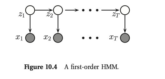 In such models our goal is usually to infer the hidden state from the observations
- A possible solution is the Hidden Markov model, where we assume that there is a underlying, hidden Markov process that generates the data, but that the observations/data are a noisy result of the underlying process.
- The main use case of graphical models is probabilistic inference, i.e we infer a set of important, hidden variables from the set of variables that we have observed. I.e we compute
- The main motivation of using graphical models is to endow the model with CI relations that reduce the computational cost. For this method to be robust we must make sure that the CI assumptions that we are making are backed by the underlying distribution and also that we know how to deduce CI relationships from a graph.
-
I-Map - (independence map) for , or that is Markov wrt , iff , where is the set of all CI statements that hold for distribution . In other words, the graph is an I-map if it does not make any assertions of CI that are not true of the distribution. This allows us to use the graph as a safe proxy for when reasoning about ‘s CI properties. This is helpful for designing algorithms that work for large classes of distributions, regardless of their specific numerical parameters .
- Note that the fully connected graph is an I-map of all distributions, since it makes no CI assertions at all (since it is not missing any edges). We therefore say is a minimal I-map of if is an I-map of , and if there is no which is an I-map of .
-
D-seperation* - First, we introduce some definitions. We say an undirected path is d-separated by a set of nodes (containing the evidence) iff at least one of the following conditions hold:
- contains a chain, or , where
- contains a tent or fork, , where
- contains a collider or v-structure, , where is not in and nor is any descendant of .
Next, we say that a set of nodes is d-separated from a different set of nodes given a third observed set iff each undirected path from every node to every node is d-separated by . Finally, we define the CI properties of a DAG as follows:
The Bayes ball algorithm (Shachter 1998) is a simple way to see if is d-separated from given , based on the above definition. The idea is this. We “shade” all nodes in , indicating that they are observed. We then place “balls” at each node in , let them “bounce around” according to some rules, and then ask if any of the balls reach any of the nodes in . The three main rules are shown in Figure 10.9. Notice that balls can travel opposite to edge directions. We see that a ball can pass through a chain, but not if it is shaded in the middle. Similarly, a ball can pass through a fork, but not if it is shaded in the middle. However, a ball cannot pass through a v-structure, unless it is shaded in the middle.
-
Markov Blanket* - The set of nodes that renders a node conditionally independent of all the other nodes in the graph is called ‘s Markov blanket; we will denote this by . One can show that the Markov blanket of a node in a DGM is equal to the parents, the children, and the co-parents, i.e., other nodes who are also parents of its children:
-